Demystifying LoRA Fine Tuning

Everything you need to learn about LoRA fine-tuning, from theory, and inner working to implementation.
Introduction
In the current era of the Language Model (LLM), we can observe that many models are being released more frequently. However, most of these models are not ready for immediate use. Therefore, we need an additional adaptation stage to customize the model according to our specific domain. This stage is called fine-tuning. During fine-tuning, the weights of the model are adjusted. Depending on how we modify the model’s weights, we can classify fine-tuning strategies into a few categories.
- Update each parameter in the model.
- Add additional parameter layers as extension layers to the current model, and update those weights while keeping the original model weights frozen. This will increase the model depth, hence increasing inference time.
- Add a dense layer to model and optimize it during adaptation, while keeping the pre-trained weights frozen.
Throughout this article, we will discuss LoRA fine-tuning, explain why it’s a more efficient fine-tuning strategy compared to other options, and list its advantages and disadvantages.
What is LoRA

Lora is short for Low-Rank Adaptation. LoRA injects trainable rank decomposition matrices into selected pre-trained layers while keeping pre-trained weights frozen.
When I first learned about LoRA, I had two questions when reading LoRA’s abstract. Those are
- What are rank decomposition matrices?
- What is the difference between LoRA, Adapters, and fine-tuning?
I will be using these two questions to explain LoRA. Let's begin!
1. What are rank decomposition matrices?
Rank decomposition matrices refer to matrices that are decomposed into a product of matrices. The goal here is to reduce the number of trainable parameters by representing large matrices using two smaller matrices. Let’s take an example. Assuming we have a 10 x 10 matrix we can represent this using 10 x r and r x 10 matrix; where r is the rank of a source matrix.
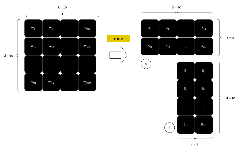
In the initial 10 x 10 matrix we had 100 elements, in AI lingo it is called trainable parameters. But after decomposition id reduces into 10 x 2 + 10 x 2 = 40 parameters. In this example, this sounds less. But in a real-world example, this is huge compute and memory save!
2. What is the difference between LoRA, Adapters, and fine-tuning?
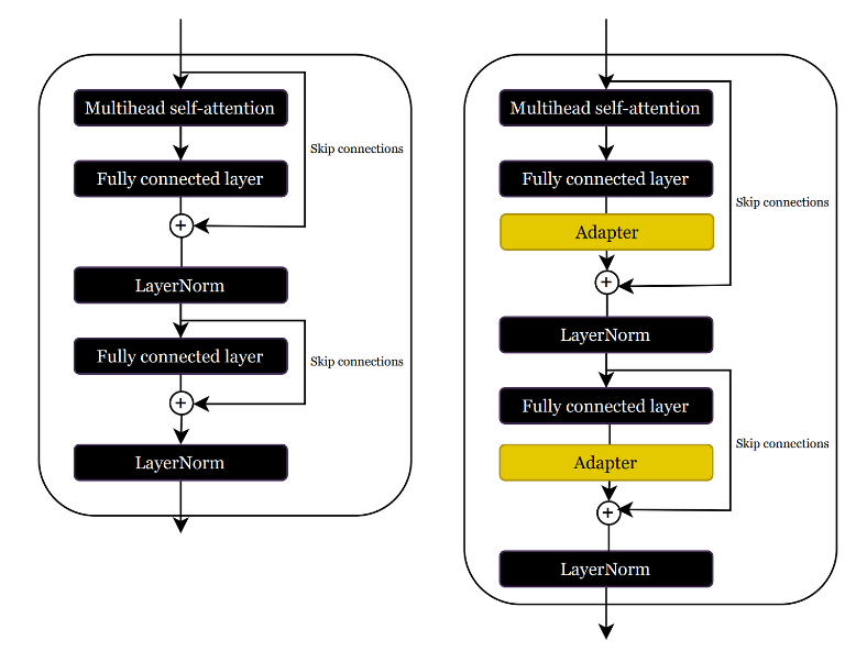
LoRA and adapters differ in their initialization process. Adapters add extra layers to the original model, which increases the neural network's depth and causes additional latency during the inference phase.
As we can see this additional latency is problematic in latency-sensitive applications. Therefore we should be aware of some additional approaches we can take to prevent it. What if we do the following,
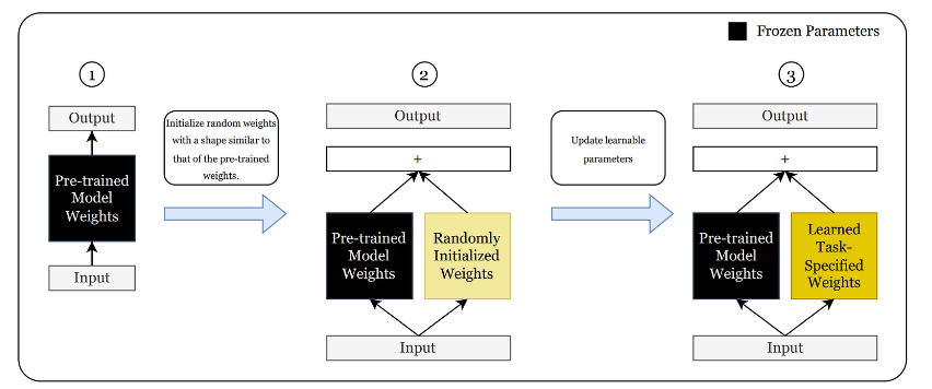
The method described in the above diagram is called regular finetuning
As shown in the third diagram, the model learns a new task while maintaining its depth by combining pre-trained and learned weights before the output layer.
But this approach again has several inefficiencies.
- The training effort is significant because we need to update the same number of parameters as the pre-trained model.
- Training a massive model for each task is not feasible due to computing and memory requirements.
To tackle these challenges, researchers have introduced LoRA, which involves reducing the learnable parameters in newly initialized layers.
3. How does LoRA reduce learnable parameter count?
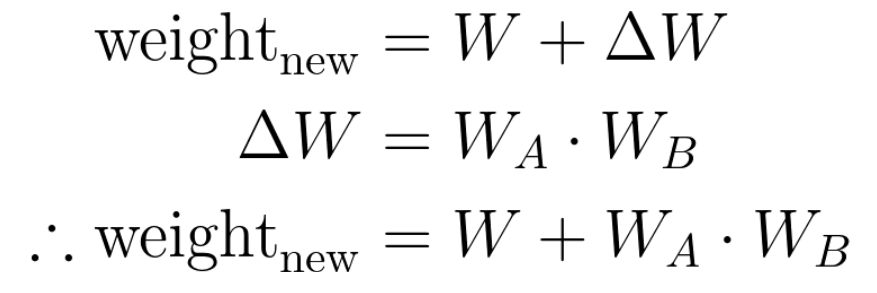
Well, that is where the previously discussed rank decomposition of the matrix comes into play. Here, instead of training large parameter matrices (∆W) what we going to do is use smaller two matrices(A & B) to approximate the large matrix (∆W).
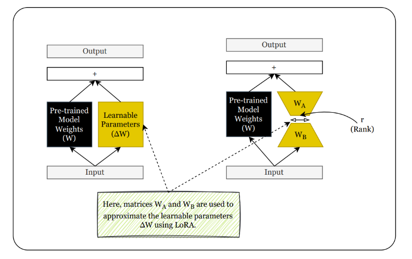
Let's assume that our W matrix has a size of 2,500 x 2,500, which means we have a total of 6.25 million parameters. Now, suppose we select r as 8. This results in having two LoRA matrices of size 2,500 x 8 and 8 x 2,500, respectively. In this case, the total number of trainable parameters is 40,000, which is a reduction of approximately 156 times.
In summary, we can represent new weights as below,
In the original paper, researchers introduced a scaling factor for ΔW. This controls the degree of weights we should put on LoRA weights. The final equation looks like this;
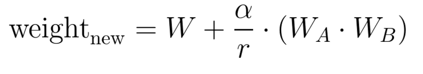
In this equation, alpha is another hyperparameter we should tune.
Practical Implementation Details

When implementing LoRA for similar tasks my go-to solution is hugging face's peft library. To install it, you can use the pip command. After the installation, we can customize the LoRA settings as per our requirements. We can choose which layers to add LoRA, LoRA Alpha, Rank parameter, and more. While selecting Alpha, it's recommended to set it to two times r.
Conclusion
LoRA fine-tuning is a type of parameter-efficient fine-tuning that involves fewer learnable parameters due to matrix approximation. One of its advantages is that we can have multiple LoRA weights specialized for different tasks, which can be swapped based on the task we are working on. The small size of LoRA makes it easy to store and swap between models. However, swapping delays could be an issue in some cases, so it's important to be mindful of when to use regular fine-tuning, adapters, and LoRA.
References
- https://arxiv.org/pdf/2106.09685.pdf (LoRA Paper)
- https://huggingface.co/blog/peft (Huggingface blog)