What is Quantization in Deep Learning: Recipe to Making Deep Learning Models Faster in Production
Introduction
Machine learning, specifically deep learning, has become increasingly popular in recent years. Thanks to advancements in hardware, companies like OpenAI can now host multi-billion parameter models to serve over 20 million people per day without any hassle. When people build super fancy models, infrastructure becomes more advanced, and vice versa.
Large organizations like OpenAI can afford the multi-million-dollar infrastructure to serve their models, as the return on investment can be a few times higher.
Let's set aside the need for expensive infrastructure and consider a more straightforward scenario: you have a new transformer model and want to decrease its inference time. Additionally, you plan to deploy the model on low-memory devices. Currently, the model takes 200ms to perform inference on a GPU and requires 1.5 GB of memory.
Let's see how we can achieve this with a mechanism called quantization .
Fixed-point vs floating-point representation
Before discussing quantization logic, it is essential to understand the internal number representation used in deep learning models. As we all know, these models are built upon a combination of numbers and operations such as addition, multiplication, derivation, etc. We can significantly improve the overall efficiency and speed of the model by making these operations more efficient and fast. But how? Well, there are several ways to do so. One way of doing this is by manipulating number representation. In computer science, there are various ways to represent real numbers, but here we will focus on two particular methods:
- Fixed-point representation: This representation has a fixed number of bits for the integer and fractional parts.
- Floating point representation: In this representation, there is no fixed allocation of bits for the integer or fractional parts. Instead, a certain number of bits are allocated for the number itself (known as the mantissa or significand), and another set of bits is reserved to indicate the position of the decimal point within that number (known as the exponent).
If you want to read more about various number formats we can use, I recommend this article.
How performance gains achieved
Typical deep neural networks require many parameters to be stored and manipulated during training and inference, resulting in significant memory and computational overhead. This can be a challenge, especially when dealing with low-memory devices. Quantization is a technique that addresses this issue by reducing the number of bits used to represent the parameters. By doing so, the memory usage of the model and computational complexity of the network is reduced, making it more efficient to train and serve.
By reducing the number of bits used to represent parameters, quantization can improve the efficiency of hardware implementations of neural networks. This is particularly important for devices with limited computational resources, such as mobile phones or embedded systems, where quantized models' reduced memory and computational requirements can lead to significant performance gains.
Most NLP transformer models are trained using a floating-point number architecture, typically FP32 or FP16, to maintain the precision of the model parameters during training. However, only a forward pass through the model is performed during inferencing to obtain the output. This provides an opportunity to convert some model parameters to low-precision to reduce memory usage and improve performance. This is the underlying logic behind quantization.
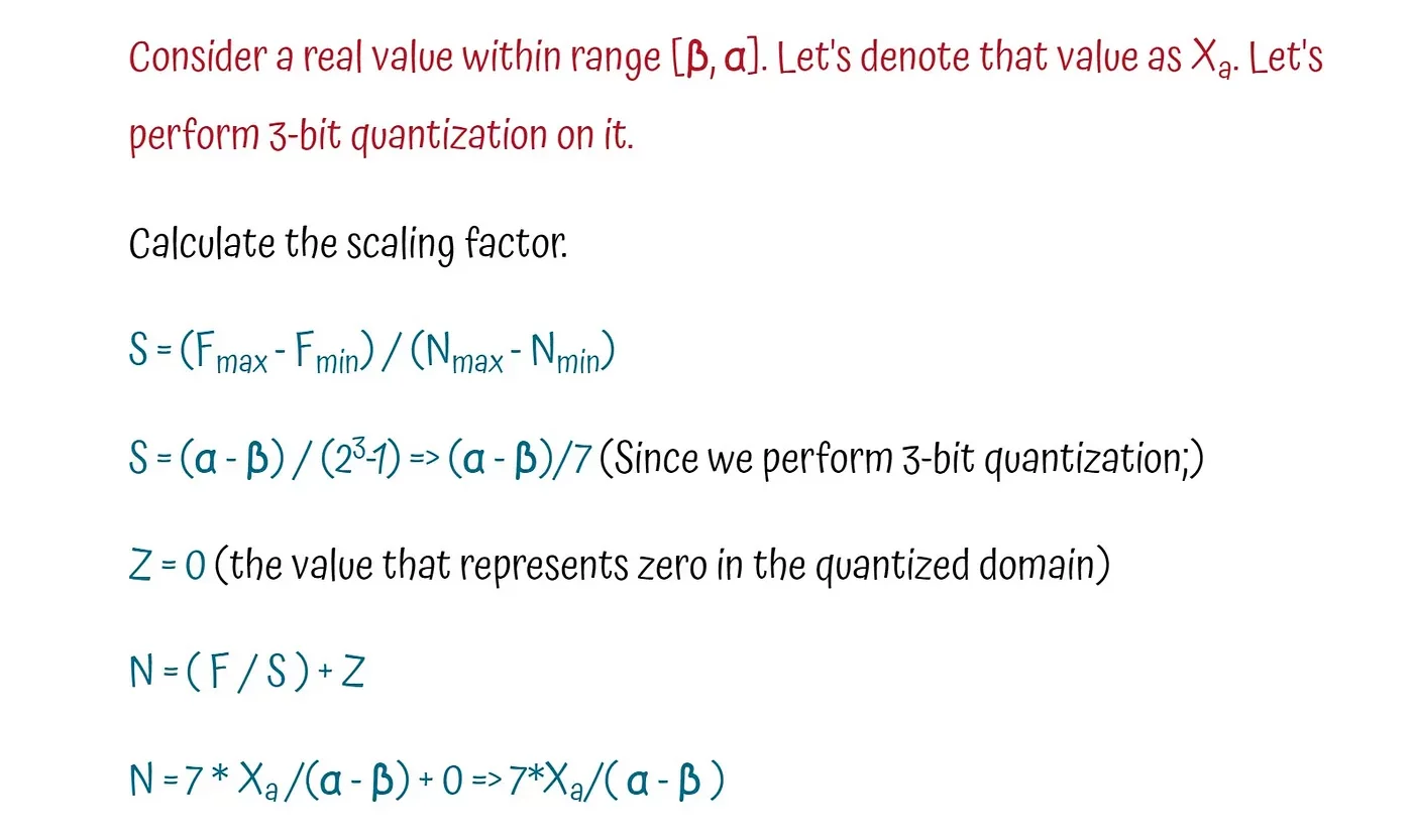
Put, quantization involves mapping high-precision values to lower-precision ones. This mapping can be described using the following equation:

N, Z, and F are the fixed point representation (Quantized representation), zero point, and floating point value, respectively. S is the scaling factor, Described in the below equation.

And we have the final equation below.

We can use the below equation to calculate the quantized number range ( N_max, N_min ) where k is the quantization bits.

If you do simple math on it, you will get N_max — N_min as 2^(k-1)
Note: Generally, we have two quantization methods that depend on the scaling logic we will use: Asymmetric Quantization and Symmetric Quantization. In this article, the technique applied is Asymmetric Quantization.
See the below example for more information.
Different approaches to quantizing deep learning models

There are typically three main approaches to quantization.
Dynamic quantization
When using dynamic quantization, this adaptation only occurs during inference, with no changes made during training. The model's weights are converted to INT8 format ahead of inference time, and the activations are also quantized. This approach is dynamic because the quantization occurs on the fly, allowing for efficient calculation of matrix multiplications using optimized INT8 functions. One of the drawbacks of this method is it still involves the conversion of activations between floating-point and integer formats, which can create a performance bottleneck.
Static quantization
We can avoid converting to a floating-point by precomputing the quantization scheme instead of computing it on the fly. Static quantization accomplishes this by examining the activation patterns on a representative data sample before inference. This results in an optimal quantization scheme that is calculated and saved. By doing this, we can eliminate the need to convert between INT8 and FP32 values, resulting in faster computations. However, static quantization requires a good data sample and introduces an additional step in the pipeline since we need to train and determine the quantization scheme before performing inference. Furthermore, static quantization does not address the precision discrepancy during training and inference, which can lead to a performance drop in the model's metrics.
Quantization-aware training
Quantization Aware Training is a technique used in deep learning to simulate the impact of quantization on a neural network during the training process. This involves computing scale factors while training the network, which represents the weights and activations of the neural network in lower precision formats.
After training, the network is modified by inserting Quantize (Q) and Dequantize (DQ) nodes into the graph. During fine-tuning, these nodes are used to simulate quantization loss and incorporate it into the training loss, making the network more robust to the effects of quantization. Simulating quantization during training improves the network's resilience to quantization, which can improve performance metrics compared to other types of quantization, like static and dynamic quantization.
How to quantize the existing Pytorch model

Using the PyTorch framework, let's apply the quantization technique to a deep learning model. To evaluate its performance, we will use the sentiment classification model from HuggingFace.
from transformers import AutoTokenizer, AutoModelForSequenceClassification,pipeline
from datasets import load_dataset,load_metric,ClassLabel

check_point = "YOUR_CHECKPOINT_HERE"

tokenizer = AutoTokenizer.from_pretrained(check_point)
model = AutoModelForSequenceClassification.from_pretrained(check_point)
In this article, we will explore the impact of quantization on inference time, memory consumption, and disk usage of a deep learning model. Let's create support functions for that.
import torch.nn as nn
import torch
from pathlib import Path

accuracy_score = load_metric("accuracy")

def compute_mem_usage(model):
 # ref: https://discuss.pytorch.org/t/gpu-memory-that-model-uses/56822/2
 param_size = 0
 for param in model.parameters():
     param_size += param.nelement() * param.element_size()
 buffer_size = 0
 for buffer in model.buffers():
     buffer_size += buffer.nelement() * buffer.element_size()

 size_all_mb = (param_size + buffer_size) / 1024**2
 return size_all_mb

def compute_metrics(pred):
 predictions, labels = pred
 predictions = np.argmax(predictions, axis=1)
 return accuracy_score.compute(predictions=predictions, references=labels)

def get_pipeline(model,tokenizer=tokenizer,device=device):
 tokenize_kwargs = {"max_length":512,"truncation":True}
 return pipeline('text-classification',model=model,tokenizer=tokenizer,device=device,**tokenize_kwargs)

def compute_accuracy(pipeline):
 preds, labels = [], []
 label_encoder = dataset.features["label"].str2int
 for example in tqdm(dataset):
   pred = pipeline(example["text"])[0]["label"]
   label = example["label"]
   preds.append(label_encoder(pred))
   labels.append(label)
accuracy = accuracy_score.compute(predictions=preds, references=labels)
return accuracy['accuracy']

def compute_size(model):
 state_dict = model.state_dict()
 tmp_path = Path("model.pt")
 torch.save(state_dict, tmp_path)
 size_mb = Path(tmp_path).stat().st_size / (1024 * 1024)
 tmp_path.unlink()
 return size_mb
Now that we have implemented the required supporting functions, it's time to quantize our model. Thanks to PyTorch, this can be achieved in just one line of code.
We use the quantize_dynamic() function, which takes the full-precision model and a list of PyTorch layer classes we want to quantize. The dtype argument specifies the target precision, in other words, the data type of our quantized model. In our case, we will use INT8 target precision.
from torch.quantization import quantize_dynamic
import torch.nn as nn
import torch

model_quantized = quantize_dynamic(model, {nn.Linear}, dtype=torch.qint8)
Let's start our experiment.
pipeline_dict = {"original_model":get_pipeline(model),'quantized_model':get_pipeline(model_quantized)}

results = []

for pipeline_name in pipeline_dict:
 loaded_model = pipeline_dict[pipeline_name].model
 mem_usage = compute_mem_usage(model=loaded_model)
 size_in_disk = compute_size(model=loaded_model)
 pipe = pipeline_dict[pipeline_name]

 start_time = perf_counter()
 accuracy = compute_accuracy(pipe)
 elapsed_time = perf_counter() - start_time

 result_dict = {
     "name":pipeline_name,
     "accuracy":accuracy,
     "elapsed_time":elapsed_time,
     "mem_usage":mem_usage,
     "size_in_disk":size_in_disk
 }

 results.append(result_dict)
Let's check out our experiment results.
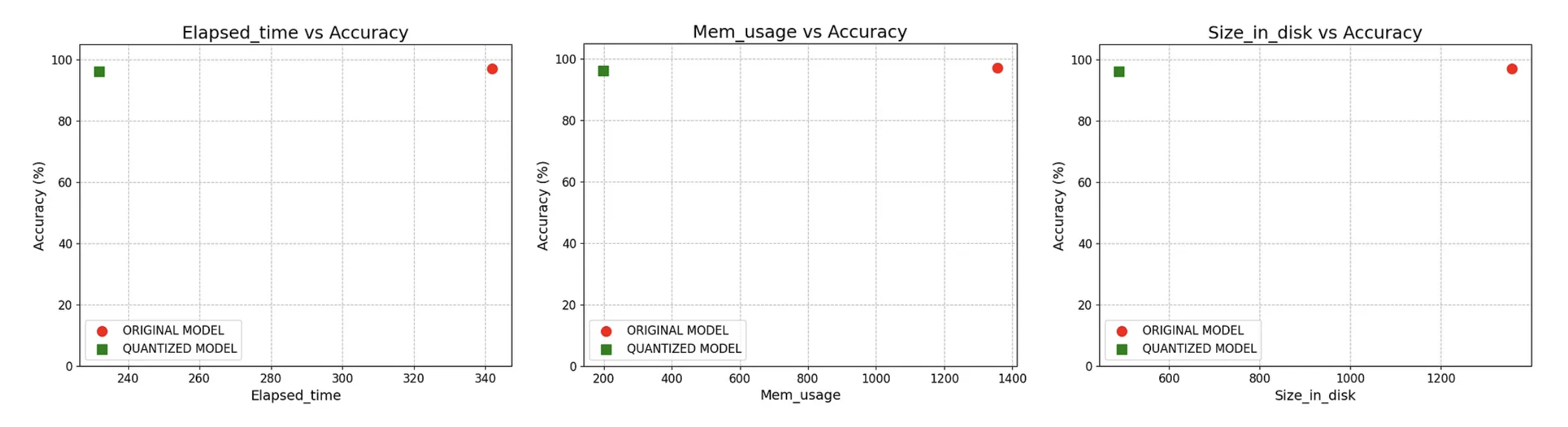
Suppose you look at the plots above. In that case, you will notice that we maintained the model's accuracy within an acceptable range (97% to 96%) while reducing the inference time by 30%, memory usage by 85%, and disk space by 64%. This significant performance improvement can benefit applications that rely on deep learning models, especially those with limited resources.
We achieved these impressive results using the dynamic quantization technique in PyTorch with just a single line of code. This simplifies the quantization process, enabling us to quickly optimize our deep learning models without sacrificing much accuracy.
End Note
While quantization can make our deep learning models faster, it's essential to understand its limitations. The scaling factor and the number of bits used for quantization must be carefully selected to balance memory usage and model accuracy. Quantization is a broad topic that this article cannot fully cover. Therefore, I recommend reading additional resources before quantizing your specific use cases. By doing so, you can make informed decisions that maximize the benefits of quantization while minimizing its potential drawbacks. You can access the code using this colab link.
Thanks for reading! Connect with me on LinkedIn.